Tip of the Week: Freezing Panes in Your Excel Spreadsheets

Microsoft Excel is a great tool for keeping data and figures organized…until, that is, you need to scroll down at all, leaving some important headers out of sight. Fortunately, there is a way to keep your headings in view: freezing the panes they are present in. Let’s go over how to do so.

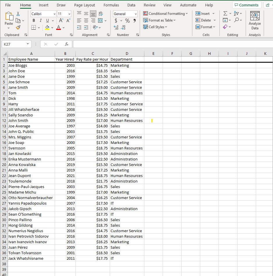
Let’s say you were working with the following data, outlining the departments each of your employees are a part of, along with when they were first hired and their current pay rate.

As you scroll down this list, you might find it useful to have a reminder of what each column is describing—and this only becomes more the case as your spreadsheets grow larger and more complicated. Luckily for us, Excel makes it easy to have certain data remain on screen.

How to Freeze Panes in Excel

Freezing a pane simply means that you’re telling Excel to keep that data visible as you scroll, and again, it’s laughably easy to do.

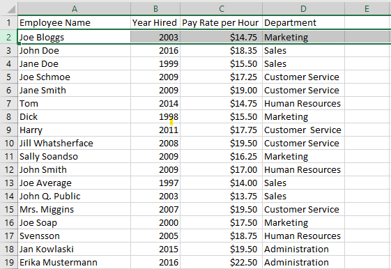
First, select the row immediately below or the column immediately to the right of the data you want frozen. In our example, since we want to keep Row 1 in sight, we’d select Row 2.

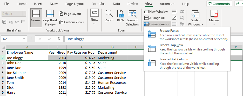
With the appropriate row or column (in this example, row) selected, you’ll next access the View tab in the ribbon and select Freeze Panes. You’ll then be presented with three options: Freeze Panes, Freeze Top Row, or Freeze First Column.

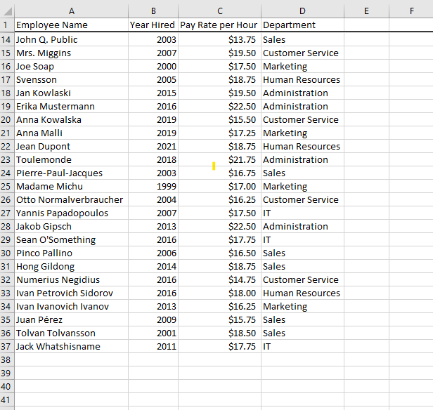
For our purposes, we’ll be selecting Freeze Panes (although Freeze Top Row would also work in this context). Once you’ve done so, you can then scroll freely, with your top row remaining in sight.

And just like that, you have continued access to critical context for your data! What else would you like to know how to do with your essential business software? Reach out to us at 1300 008 123 and let us know, or to learn more about how we can generally make your IT maintenance a non-issue for your business.